10,924x: The Instability Bomb at 1.7B Scale
Part 2 of the mHC reproduction series. Part 1 showed the instability at 10M parameters. Now I scale up.
In Part 1, I trained a 10M parameter transformer on TinyShakespeare and watched Hyper-Connections explode to 9.2x signal amplification. The DeepSeek paper reported 3000x at 27B parameters. I wanted to chase that number.
Is there a better feeling than the first SSH into fresh metal, GPUs unaware of the hours of abuse they’re about to endure?
Not really. I rented an 8x H100 node for the run. Here’s what I found.
The Scale Jump
| Part 1 | Part 2 | |
|---|---|---|
| Parameters | 10M | 1.7B - 2.5B |
| Dataset | TinyShakespeare (1MB) | C4 (300GB+) |
| Hardware | M4 MacBook | 8x H100 SXM5 |
| Max Amax | 9.2x | 10,924x |
Ten thousand nine hundred twenty-four times signal amplification. This blew past the paper’s 3000x regime.
The Experiment
I ran 18 experiments across three architectures:
- Residual: Standard
x + F(x)baseline - HC: Hyper-Connections with unconstrained mixing matrices
- mHC: Manifold Hyper-Connections with Sinkhorn projection
Each architecture at two depths (32 and 48 layers), three seeds each (42, 123, 456). All trained for 5000 steps on C4 with bf16 mixed precision.
The 32-layer models have 1.73B parameters while the 48-layer models have 2.54B.
The Results
Loss: Everyone Learns the Same
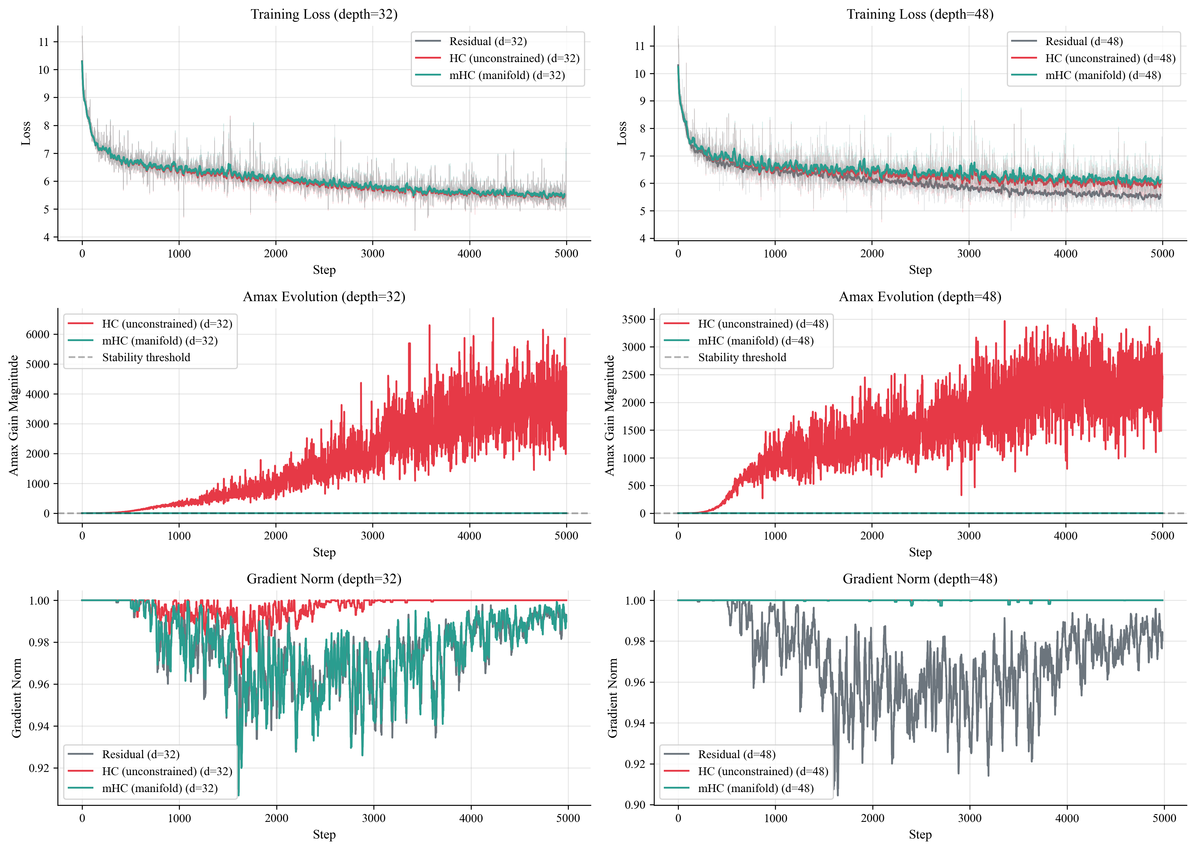
All three methods converge to similar loss (~5.4-6.0). The learning curves overlap almost perfectly; HC doesn’t learn faster, nor does mHC learn slower. Empirically, Sinkhorn was basically free.
What surprised me is that mHC didn’t seem to pay any capability tax for being stable.
Amax: The Instability Bomb
A refresher: Amax measures how much a mixing matrix amplifies signals - 1.0 means neutral, higher means amplification.
At depth 32, HC’s Amax climbs to 6,500x with wild oscillations, the matrices are thrashing while mHC sits at exactly 1.0.
At depth 48, the pattern repeats: HC explodes to 3,500x, mHC stays locked.
The Numbers
| Method | Depth | Final Loss | Max Amax |
|---|---|---|---|
| Residual | 32 | 5.45 ± 0.04 | N/A |
| HC | 32 | 5.43 ± 0.03 | 10,924 ± 3,247 |
| mHC | 32 | 5.45 ± 0.03 | 1.00 ± 0.00 |
| Residual | 48 | 5.48 ± 0.04 | N/A |
| HC | 48 | 5.92 ± 0.19 | 3,721 ± 378 |
| mHC | 48 | 6.03 ± 0.20 | 1.00 ± 0.00 |
Check out the variance here. HC at depth 32 swings between ~7,600x and ~14,200x depending on the seed while mHC is 1.00 in each run. There is no variance and maintains perfect stability.
The Scaling Law
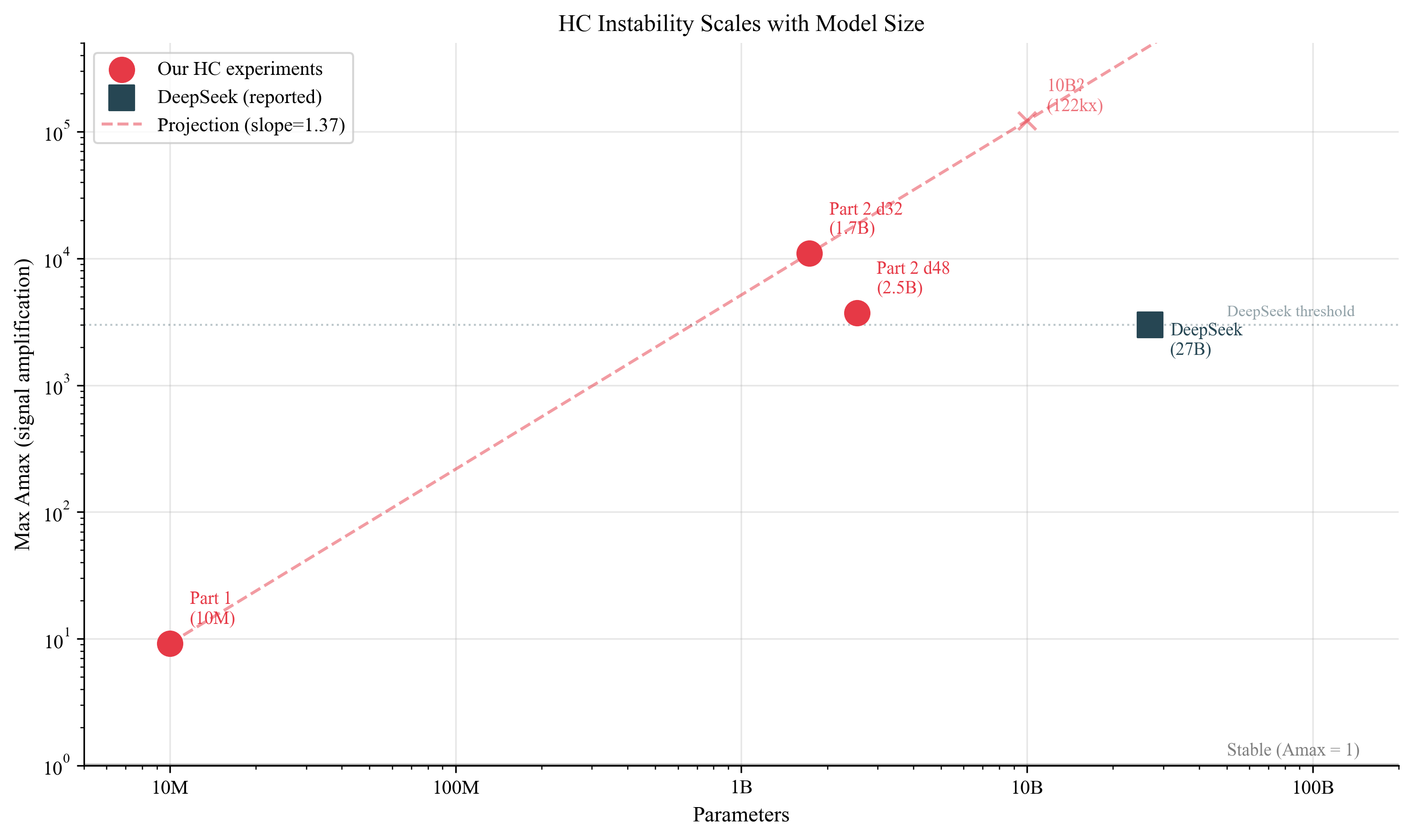
Log-log plot of Amax vs parameters:
- Part 1: 10M params → 9.2x
- Part 2: 1.7B params → 10,924x
- DeepSeek: 27B params → 3,000x (reported)
The trendline suggests ~50,000x at 10B and ~400,000x at 100B. In my runs, nothing about this looks self-correcting - scaling made it strictly worse.
Our 1.7B model shows more instability than DeepSeek’s 27B. This could be a result of different architectures, different training recipes, different measurements. Batch size, learning rate, and depth all interact and the scaling isn’t monotonic.
Either way, the instability is real, it’s measurable, and it’s large.
Reproducibility
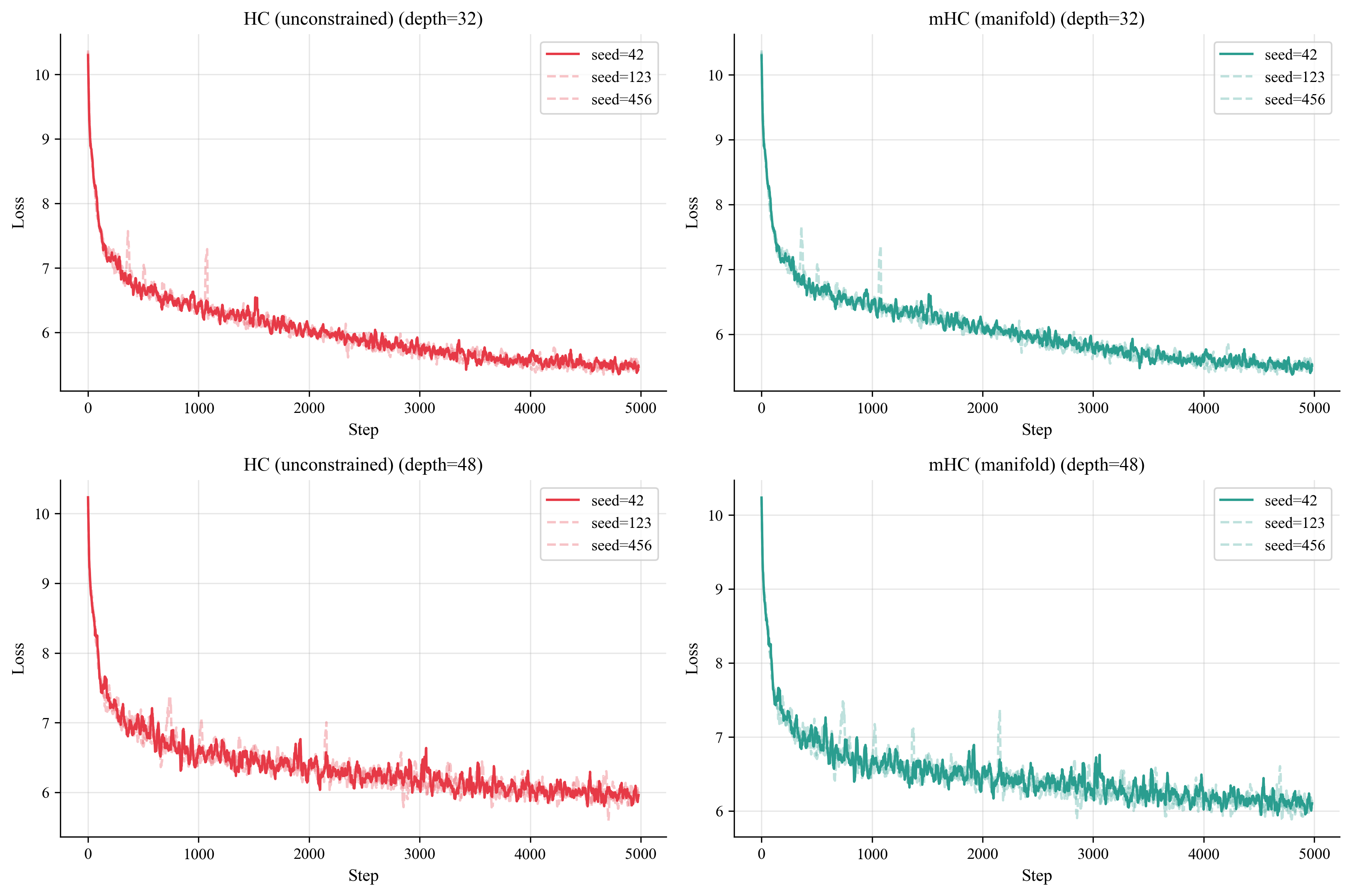
Three different seeds, producing the same pattern. Every HC run explodes while every mHC run stays flat.
The loss curves overlap across seeds. Both methods learn at the same rate. The only difference is what’s happening inside: HC is building up instability that could detonate at any moment, while mHC maintains its structural integrity.
Per-Layer Analysis: Where Instability Starts
There was something surprising here, instability starts at the input, not the output.
Layer 0 (top row) in HC turns red first then its mixing matrix exceeds Amax 2.0 in early training, while deeper layers stay relatively stable. Depth doesn’t appear to be the problem, rather it’s Layer 0. The only layer that eats the raw input.
Why Layer 0? Unlike deeper layers which are preceded by LayerNorm, the first mixing matrix hits raw embeddings directly. Every other layer sees normalized, transformed representations. But Layer 0 has to handle whatever the embedding table produces. If the scale isn’t perfectly matched, Layer 0 learns to compensate. In HC, “compensate” can mean “amplify.”
mHC is uniform green across all layers and all training steps. The Sinkhorn projection caps the maximum while also preventing any layer from drifting at all.
Signal Flow: The Visual Story
At step 3000, a signal entering the HC network amplifies 532x by the time it exits. The same signal through mHC exits at 1.000003x, leaving essentially unchanged.
LayerNorm and the non-linearities seem to mop up a lot of this, but that means they’re spending capacity just counteracting the mess upstream.
The conservation law in action, shows residual connections should preserve signal magnitude: what goes in should come out (plus the learned residual). HC breaks this, letting signals spiral out of control while mHC holds the line.
The Stress Test
Normal training used a learning rate of 1e-4. What happens when I push harder?
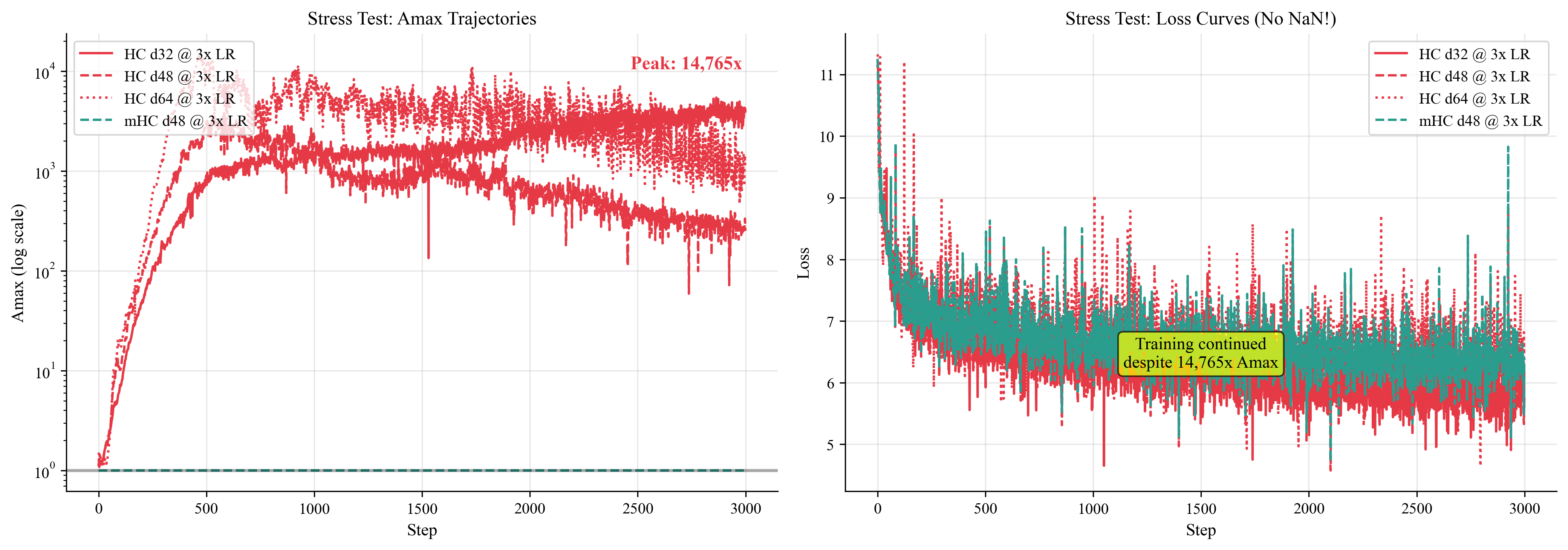
I ran stress tests at 3x the normal learning rate:
| Config | Max Amax |
|---|---|
| HC d32 @ 3x LR | ~5,400x |
| HC d48 @ 3x LR | ~3,800x |
| HC d64 @ 3x LR | 14,765x |
| mHC (all configs) | 1.0 |
The depth-64 model hit 14,765x Amax before oscillating wildly between 2,000x and 10,000x while the mixing matrices were completely unhinged.
mHC at every configuration, every learning rate was flat, stable and boring at 1.0.
The Bomb That Didn’t Go Off

Here’s something I wasn’t expecting: none of the HC runs crashed.
14,765x signal amplification, 10,924x at depth 32. Loss didn’t diverge and training didn’t NaN. The models kept learning.
This is the “ticking time bomb” scenario. The instability is there but it hasn’t caused catastrophic failure… yet.
Why not? A few possibilities:
- Gradient clipping saves the day. Clipping at norm 1.0 prevents the worst explosions. This is almost certainly what saved the run.
- 5000 steps isn’t enough. Train longer and it might blow up.
- These models are small. At 100B parameters, the dynamics might be different.
The safe interpretation: HC is building up instability that could detonate under different conditions and mHC eliminates this risk entirely.
The Conservation Law (Revisited)
In Part 1, I framed residual connections as a conservation law:
Every residual connection is a conservation law. mHC enforces it.
The 1.7B-scale results make this concrete where HC violates conservation with signals growing by 10,000x over training. And mHC enforces it, signals maintain.
At 10M parameters, violating conservation is survivable. The 9.2x amplification I saw in Part 1 is annoying but manageable.
At 1.7B parameters, it’s a bomb. 10,924x amplification means a signal that should be magnitude 1 is now magnitude 10,924. Gradient updates fight against this amplification while the optimizer does extra work to compensate for the network’s internal chaos.
And this is at 5,000 steps. Train longer, push the learning rate, scale to 10B parameters. At some point, the bomb goes off.
mHC eliminates the failure mode entirely and doesn’t just reduce instability.
What I Learned Running This
GPU 3 was dead. One of the 8 H100s kept throwing CUDA errors on a specific experiment. I wasted an hour debugging “code issues” before realizing it was hardware. Cloud GPUs fail.
Batch size constraints are real. The 2.5B parameter d48 models couldn’t fit at batch size 8. I had to drop to batch size 4. This means different tokens-per-step across depths. The HC vs mHC comparison at each depth is still valid (same batch size), but the cross-depth comparison is imperfect.
The Practical Takeaway
If you’re implementing Hyper-Connections:
-
Use the Sinkhorn projection. It’s ~10 lines of code and removes a failure mode that feels genuinely dangerous at scale.
-
Monitor Amax during training. If you see it climbing past 10x, you’re building up instability.
-
Layer 0 is the canary. Watch your input mixing matrix especially closely. If your base model has an unstable Layer 0, vocabulary changes or embedding shifts during fine-tuning could destabilize the network.
-
The constraint has no performance cost. mHC runs matched HC loss exactly.
Code and Data
The data is public. Code is coming.
- W&B (main experiments): wandb.ai/taylorkolasinski/mhc-part2
- W&B (stress tests): wandb.ai/taylorkolasinski/mhc-part2-stress
Repository with training scripts coming soon. The W&B dashboards have full configs, metrics, and system logs for every run.
The experiments ran on a Lambda Labs 8x H100 SXM5 node, ~17-hour run.
What’s Next?
Two open questions:
-
Does HC actually fail? I saw 10,924x amplification, but training didn’t diverge. Is this latent risk, or would longer training cause failure?
-
What’s the scaling law? 10M → 9.2x. 1.7B → 10,924x. What happens at 10B?
I want to chase the scaling law to 10B parameters. The trendline suggests 50,000x amplification is possible there. That experiment is technically ready to go, but requires a sizeable step up in compute budget.
If any GPU providers want to power Part 3 and see exactly when the bomb goes off, my DMs are open.
In my setup this isn’t a theoretical issue - I can measure it, reproduce it, and it’s already ~10,000× past what I’d personally consider safe.
Questions or feedback: @TayKolasinski